Mock Community Generation

Creation of test communities

Background

In order to make the differences between the metrics presented on this site more apparent, it would be helpful to have a standard mock community that can be used.

Here, I will make two sets of 3 communities - one set that differs in sequencing depth, and another that differs in evenness.

True community with known abundances

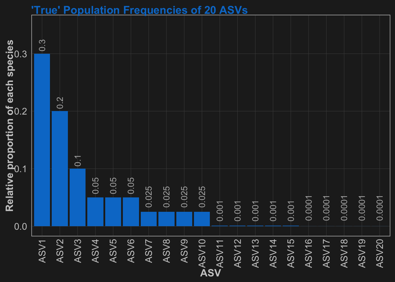
First, I will define a true population that mimics a typical microbial community population that has a “long tail” distribution. Our community will have 20 total members, 10 of which are above 1% abundance, and the other 10 are below 1% in abundance.

asv_probabilities = c(0.3, 0.2, 0.1, rep(0.05, 3), rep(0.025, 4), rep(0.001, 5), rep(0.0001, 5))
names(asv_probabilities) <- paste("ASV", 1:length(asv_probabilities), sep = "")

Each species is named with “ASV” plus a number that increases with decreasing abundance. Don’t worry if you are not familiar with ASVs are what they mean. For now, just think of them as simply the microbial species names.

Different sequencing depths (mock community #1)

Starting with this distribution of the true community, let’s take 3 samples at depths of 10,000, 1,000 and 100. This is done with replace=TRUE to simulate a very (infinitely?) large population.

Sample_1 = table(sample(x=names(asv_probabilities), size=10000, replace=TRUE, prob=asv_probabilities))
Sample_2 = table(sample(x=names(asv_probabilities), size=1000, replace=TRUE, prob=asv_probabilities)) 
Sample_3 = table(sample(x=names(asv_probabilities), size=100, replace=TRUE, prob=asv_probabilities))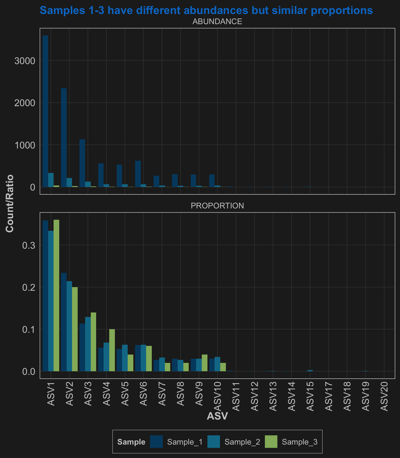

Different diversity/evenness (mock community #2)

Next, we will take these same 20 species and define different true proportions to sample from. These next three communities will have decreasing evenness from 1) all 20 perfectly even, 2) ten species with 10x more abundance than the other 10, and 3) two species with 100x more abundance than the other 18 species.

Then, each will be sampled 10,000 times to give us the same sequencing effort.

Sample_4 = table(sample(x=paste("ASV", 1:20, sep = ""), size=10000, replace=TRUE, prob=c(rep(1,1), rep(1,19))))
Sample_5 = table(sample(x=paste("ASV", 1:20, sep = ""), size=10000, replace=TRUE, prob=c(rep(10,10), rep(1,10))))
Sample_6 = table(sample(x=paste("ASV", 1:20, sep = ""), size=10000, replace=TRUE, prob=c(rep(100,2), rep(1,18))))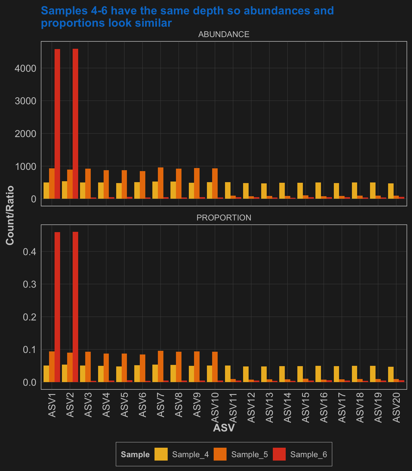

Combining into one dataset

Now, these 6 samples can be made into an “ASV table” with samples in columns, and species names in rows.

d = list(Sample_1, Sample_2, Sample_3, Sample_4, Sample_5, Sample_6)
names(d) = c("Sample_1", "Sample_2", "Sample_3", "Sample_4", "Sample_5", "Sample_6")

mock_community = bind_rows(d, .id = "SAMPLE") %>%
    pivot_longer(cols = c(everything(), -SAMPLE), names_to = "ASV") %>% 
    mutate(value = as.numeric(value), value = ifelse(is.na(value), 0, value)) %>% 
    pivot_wider(names_from = SAMPLE, values_from = value)  %>%
    mutate(ASV = fct_relevel(ASV, gtools::mixedsort(unique(as.character(.$ASV))))) %>% 
    arrange(ASV)

Same Evenness, Differing Depth or Same Depth, Differing Evenness
ASV	Different Depth			Different Evenness
	Sample_1	Sample_2	Sample_3	Sample_4	Sample_5	Sample_6
ASV1	3589	334	36	503	934	4584
ASV2	2337	214	20	536	897	4594
ASV3	1134	129	14	504	926	42
ASV4	559	68	10	498	875	47
ASV5	533	63	4	480	873	56
ASV6	624	63	6	513	848	40
ASV7	268	33	2	531	955	50
ASV8	302	27	2	524	926	44
ASV9	300	30	4	494	936	50
ASV10	300	34	2	510	932	44
ASV11	14	0	0	511	92	45
ASV12	8	0	0	480	79	46
ASV13	11	1	0	475	89	42
ASV14	8	0	0	491	85	34
ASV15	6	3	0	492	101	46
ASV16	0	0	0	502	80	52
ASV17	1	0	0	485	87	47
ASV18	1	0	0	502	97	36
ASV19	3	1	0	496	95	44
ASV20	2	0	0	473	93	57

OK, everything looks good. This dataset can now be saved in order to use it in other pages as necessary.