Simpson’s Diversity

By Hand

What are the chances of sampling the same thing twice?

Published

December 27, 2021

There are three different (but mathematically related) values for Simpson Diversity¹. All are per-sample alpha-diversity metrics with the aim of putting a quantitative metric to the distribution or “evenness” of the members of a sample. High evenness means that the community members are in similar proportions to one another, and low evenness (or high unevenness) indicates that there are one or a few community members that dominate.

It is common for publications to say something like “the Simpson’s Diversity was x”, but it is important to understand which Simpson’s measure is being referred as different groups use these names interchangeably. I find it best to refer to them by the variables \(\textcolor{#037bcf}{D}\), \(\textcolor{#037bcf}{1-D}\), or \(\textcolor{#037bcf}{\frac{1}{D}}\). We’ll go over these below, but just keep in mind that \(\textcolor{#037bcf}{D}\) is an unevenness metric, while \(\textcolor{#037bcf}{1-D}\) and \(\textcolor{#037bcf}{\frac{1}{D}}\) are evenness metrics.

Below, we will use the mock communities to test our calculations. Samples 4-6 will be useful here as they were designed to have high (Sample 4), medium (Sample 5) and low (Sample 6) evenness.

Simpson’s Index (D)

The Simpson’s Index, or simply \(\textcolor{#037bcf}{D}\), is the probability of randomly picking two species that are the same. It is a metric from 0 to 1, and the closer to 1, the less diverse (or more uneven) your sample is. A value of 1 means you have a very high probability of picking the same group, which means you have one species that is very dominant. \(\textcolor{#037bcf}{D}\) works on species proportions rather than abundances. Because of this, our communities are considered “infinitely large”, and removing the individual in the first pick doesn’t change the probabilities of what you will get in the second pick. This is easily done in the sampling method by sampling “with replacement”. If we didn’t sample with replacement then the odds of what you will get in pick 1 will not be the same as in pick 2.

\(\textcolor{#037bcf}{D}\) will always be above 0, because there is always a chance of picking the same thing twice. The theoretical minimum value possible is \(\textcolor{#037bcf}{\frac{1}{S}}\) (where \(\textcolor{#037bcf}{S}\) is the richness). The theoretical maximum of \(\textcolor{#037bcf}{\frac{1}{S}}\) could equal 1 if you only had one species.

The value of \(\textcolor{#037bcf}{D}\) is just the sum of the squared proportions (Pi) for each individual. While we are at it, let’s also calculate the theoretical minimum \(\textcolor{#037bcf}{D}\) for each sample by taking \(\textcolor{#037bcf}{\frac{1}{S}}\).

D = mock_community %>%
  pivot_longer(cols = c(everything(), -ASV), names_to = "SAMPLE", values_to = "ABUNDANCE") %>%
  filter(ABUNDANCE > 0) %>% 
  group_by(SAMPLE) %>%
  mutate(Pi = ABUNDANCE / sum(ABUNDANCE)) %>%
  mutate(Pi2 = Pi ^ 2) %>%
  summarise(D = sum(Pi2), MIN_D = 1 / n(), S = n())

Note, the filter(ABUNDANCE > 0) is only needed for the MIN_D and S calculations and not to get D.

Sample	D	MIN_D	S
Simpson's D (unevenness)
Sample_1	0.210	0.053	19
Sample_2	0.190	0.077	13
Sample_3	0.207	0.100	10
Sample_4	0.050	0.050	20
Sample_5	0.084	0.050	20
Sample_6	0.422	0.050	20

We get the expected values when running on the mock community, where the unevenness increases from Sample 4 to Sample 6. In the most uneven sample (Sample 6) we have a 42% chance of picking the same species twice. In our “perfectly even” Sample 4, we see that \(\textcolor{#037bcf}{D}\) is very close to the theoretical minimum of \(\textcolor{#037bcf}{\frac{1}{S} = \frac{1}{20} = 0.05}\), or only a 5% chance of getting the same species twice.

There are changes in Samples 1-3, but they are more subtle. Even though the true population had an true evenness value, we get an apparent drop in evenness as the sampling depth goes down and we lose the low-abundance samples giving an artificial bump in the proportions of the higher abundance samples.

Simpson’s Diversity Index (1 - D)

If \(\textcolor{#037bcf}{D}\) is the probability of picking the same species twice, then \(\textcolor{#037bcf}{1-D}\) is the probability of picking a different species This is a measure of evenness, where the closer to 1 the more even your population is.

The possible values are opposite for \(\textcolor{#037bcf}{D}\), with it never getting to 1, but with 0 possible under extreme conditions. The theoretical maximum is \(\textcolor{#037bcf}{1 - \frac{1}{S}}\).

Starting with our D dataframe from above,

D = D %>%
  mutate(`1-D` = 1 - D)

Sample	D	MIN_D	1-D	S
Simpson's 1-D (evenness)
Sample_1	0.210	0.053	0.790	19
Sample_2	0.190	0.077	0.810	13
Sample_3	0.207	0.100	0.793	10
Sample_4	0.050	0.050	0.950	20
Sample_5	0.084	0.050	0.916	20
Sample_6	0.422	0.050	0.578	20

So, just the opposite conclusions of \(\textcolor{#037bcf}{D}\) where our chances of picking two different species is slightly lower than if they were in equal proportions.

Vegan Simpson

This is the value returned when running diversity(index = "simpson") in vegan². And, since it uses vegan under the hood, what phyloseq³ gives as Simpson when running estimate_richness().

Here it is run through vegan giving the same values as our 1-D column in Table 2 above.

V = mock_community %>%
  column_to_rownames("ASV") %>%
  as.matrix() %>%
  t() %>%
  vegan::diversity(index = "simpson")

Sample	Simpson
Vegan Simpson
Sample_1	0.790
Sample_2	0.810
Sample_3	0.793
Sample_4	0.950
Sample_5	0.916
Sample_6	0.578

Simpson’s Reciprocal or Inverse Index (1 / D)

This is the the inverse of \(\textcolor{#037bcf}{D}\), telling us the number of equally common species that will produce the observed \(\textcolor{#037bcf}{D}\). That is kind of a mouthful, so another way to think about it is if your \(\textcolor{#037bcf}{D}\) is 25% (or 1/4), you can get that value if you had 4 individuals in equal proportions. So, \(\textcolor{#037bcf}{1/D}\) is getting at a number of individuals in the same units as your original values (“species” in our case). The higher the value, the more equally abundant individuals you have and therefore a higher evenness.

D = D %>%
  mutate(`1/D` = 1 / D)

Sample	D	MIN_D	1-D	1/D	S
Simpson's 1/D (evenness)
Sample_1	0.210	0.053	0.790	4.771	19
Sample_2	0.190	0.077	0.810	5.251	13
Sample_3	0.207	0.100	0.793	4.826	10
Sample_4	0.050	0.050	0.950	19.977	20
Sample_5	0.084	0.050	0.916	11.938	20
Sample_6	0.422	0.050	0.578	2.372	20

The theoretical minimum is 1, and maximum is just \(\textcolor{#037bcf}{S}\). If the value is close to 1, this means there is a single dominant species influencing the calculations. Values closer to \(\textcolor{#037bcf}{S}\) show the species abundances are more even.

Let’s put our numbers into perspective where the X is \(\textcolor{#037bcf}{1/D}\), and the range for each sample goes from 1 to \(\textcolor{#037bcf}{S}\):

D %>%
  ggplot(aes(x = SAMPLE, y = `1/D`, fill = SAMPLE)) +
    #geom_col() +
    scale_fill_manual(values = sample_palette) +
    geom_crossbar(aes(ymin = 1, ymax = S), width = 0.9, color = "gray30") +
    geom_point(size = 10, color = "gray30", pch = 4, stroke = 2) +
    theme(legend.position = "none")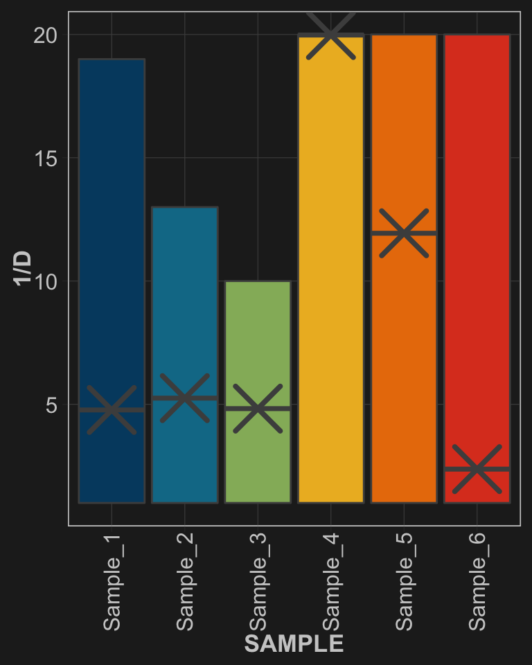

Samples 1-3 have similar proportions and also have similar Inverse Simpson values. Samples 4-6, however, show very different results with Sample_4 (perfect evenness) being at the maximum theoretical value, and Sample_6 (only two dominant ASVs) being down around 2.

Vegan invsimpson

Similarly, This is the value returned when running diversity(index = "invsimpson") in vegan and what phyloseq gives as InvSimpson when running estimate_richness().

V = mock_community %>%
  column_to_rownames("ASV") %>%
  as.matrix() %>%
  t() %>%
  vegan::diversity(index = "invsimpson")

Sample	invsimpson
Vegan Simpson
Sample_1	4.771
Sample_2	5.251
Sample_3	4.826
Sample_4	19.977
Sample_5	11.938
Sample_6	2.372